Modelling

Introduction

We now have a better understanding of our data. Before going onto training a model, we must better understand the problem our user is facing. Only then can we start modelling.

This section goes over the process of getting from understood data to working model.

From business problem to modelling task

Let’s go back to our business problem:

Business Problem

We are an energy distribution company. As such, we deal with the consumption of energy throughout our grid. We don’t know how said consumption will evolve in the future, and it would help us to know.

We want – equipped with our new understanding of the context, constraints and needs of our business – to solve this problem. To solve it, we first need to translate it into a modelling task, i.e. to formulate it in terms of input, machine learning model and output.

There are several correct ways to do so. In our case, we take inspiration from the way the ENTSO-E names their own prediction, i.e – Day-ahead Total Load Forecast – and assume that they forecast the consumption between t and t + 1h using the data available a a full day before t.¹

Our modelling task could then be formulated as such:

Modelling task

At time t, given all the load data prior to t, predict the load in MW at t + 24h

graph LR
  A[Prior hourly-load data] --> B[ML model] --> C[Hourly-load in 24h]

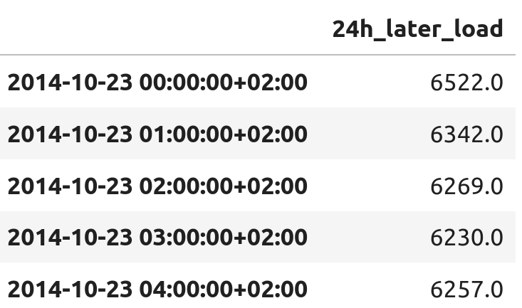
We wrangle the data to better represent our modelling task. That is, each row’s index is now the timestamp t, and the target – called 24h_later_load – is the actual load [MW] between t + 24h and t + 24h + 1h.

from datetime import timedelta

df = df.set_index(df.index - timedelta(hours=24))
df = df.rename(columns={'Actual Load': '24h_later_load'})
df.head()

Image title — A data model fitting our modelling task.

Where to start

Where can we even start solving this ?

Let’s stand back a little bit and think about the choice in front of us. We’re about to build some machine learning model to solve our modelling task. We can go with an ARIMA model, a transformer-based approach, or even the latest NeurIPS paper.² Really, we have to choose how complex³ our first attempt at modelling should be.

Young and freshly out-of-college, we could let our excitement win and dive straight into implementing the most complex ML-based time-series prediction model. Assuming that surely complexity and modernity are synonymous with performance, right? This would be a mistake, as our goal is not to build the best model, but to answer the need of the business.⁴

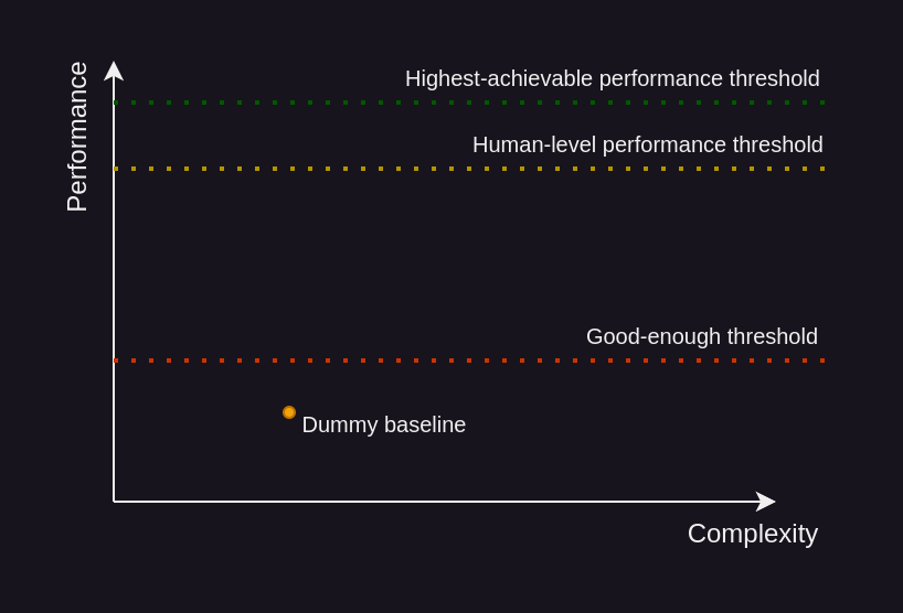
There is such a thing as good-enough

Most industry problems have a “this is good-enough” threshold.

This “good-enough” threshold is the lowest performance that satisfies the needs of the business. It’s often hard to express in hard numbers, and comes from understanding the business needs. Often, you will end up with an approximation acting as a proxy, meaning that a model performing up to that standard should fulfill those needs.⁵

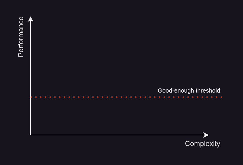
Back at our initial choice, and we can either start simple or complex.

We really should start simple, for many reasons:

A simple solution might place us above the “good-enough” threshold, saving us a lot of work.
It is often difficult to know where the “good-enough” threshold should be. Building a simple approach and getting user feedback on it allows us to place it above or below that approach’s performance.
A simple solution is an effective benchmarking tool against which we can rank other solutions.
A simple solution is a good sanity check that our understanding of our problem and data sources are sound.
Let’s assume we started with a complex solution. The cost (in time and ressource) to go onwards with it – in terms of industrialization, deployment and maintenance – would far outweigh the cost of trying a simple solution. And if a simple solution was acceptable, then we’d go for the simple solution. Hence, even if we started from a complex approach, we’d build the simple approach just to check and justify the complex approach.
It’s easier to start simple and add complexity step by step.

Please

Start simple⁶

Wonderful, let’s say we listened and started with a simple approach – a dummy baseline. Unfortunately, the user is not satisfied – i.e. the business need is not answered, and we’re below the “good-enough” threshold.

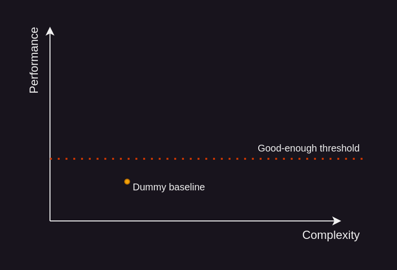
From that point on, we can add complexity step-by-step, till we – hopefully – surpasses the “good-enough” threshold.

As we try different approaches, we should be mindful that we are facing a performance upper-bound.

Performance upper-bound

Most prediction problems have a performance upper-bound.

That is, there is in almost all cases some amount of randomness when predicting the future from a given set of observations. A direct consequence of that is that regardless of how good your model is, you will not be able to perfectly predict the future.

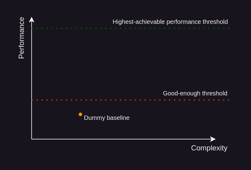
All you can do is hope that this upper-bound is above the “good-enough” threshold. Akin to the “good-enough” threshold, this upper-bound is rarely available to us. What we can do is measure the human-level performance on that task, which would give us a lower-bound to that upper-bound.

Now that we’ve talked extensively about where to start, let’s actually start modelling.

Dummy Baseline

Back to our wrangled dataset:

We’ll start with the following dummy baseline:

Dummy baseline

Predict that the hourly-load at time t + 24h is yesterday hourly-load at the same hour, i.e. the hourly-load at time t - 24h ⁷

Build, test and plot the dummy baseline

from datetime import timedelta
from sklearn.metrics import mean_absolute_percentage_error
import plotly.express as px

# Enrich the data with the 24h_ago_load
df = df.asfreq('h') # Enforce an hourly frequency
df['24h_ago_load'] = df['24h_later_load'].shift(48)

# Only consider the last year
with_load_latest_ts = df[~df['24h_later_load'].isna()].index.max() 
df = df[df.index >= with_load_latest_ts - timedelta(days=365)]

# Build y_true and y_pred
df = df.dropna()
y_true = df['24h_later_load']
y_pred = df['24h_ago_load']
print(f'MAPE over the last year: {mean_absolute_percentage_error(y_true, y_pred) * 100:.2f}%') 
# MAPE over the last year: 8.97%

# Plot the last month
df = df[df.index >= df.index.max() - timedelta(days=30)]

fig = px.line(
    df, x=df.index, y=['24h_later_load', '24h_ago_load'], 
    title='Actual load and dummy forecast over the last month',
    labels={'index': 'Date', 'value': 'Load [MW]', 'variable': ''}
)

fig.for_each_trace(lambda t: t.update(name={'24h_later_load': 'Actual load', '24h_ago_load': 'Dummy forecast'}[t.name]))

Approaching our problem like this yields the following results over the past year:

Yearly-MAPE [%]	Model
10.8	ENTSO-E forecast
8.97	Dummy baseline

Now, that’s surprising – I’d have expected our dummy forecast to be worse than the official one. It is likely they are relying on less informations than us to forecast the future loads.¹ Still, we can work off this baseline to further improve our approach.

LightGBM to the rescue

I love lightgbm.

It is easy to deploy, battle-tested, fast to iterate one and performs extremely well. ⁷

Whenever I am solving a task where it might give an answer, I try it. I’ll only whip out the big guns – i.e. deep learning – if I really need it.

Let’s continue our modelling journey by building upon it.

Walk-forward validation

Now, before we dive into training – and testing – an LightGBM-based model – any model really – we should take a step back and think about what we’re about to do.

Our problem looks like a classic regression task. As such, one might feel enclined to follow the classic regression-task flow, i.e.

Randomly divide the data into train and test sets
Train some model on the train set
Test that trained model on the test set

If we did that, we would end up with an great-performing model on the test set. We would happily go onto making it available to our users, but then that model would underperform.

Why?

Because we’re not solving a typical regression task, we’re dealing with timeseries. Whenever we are training/testing a model, our testing conditions should mimic as closely as possible our real-life conditions. Essentially, we’re assuming that the test data has been drawn from the same distribution as our real-life data. If that assumption is wrong, then any performance on the test set might not correlate to our model’s real-life performance.⁸

Testing should be real-life

Testing conditions should be as close as possible to real-life conditions.

How does that impact us in our time-series prediction task? Well, by randomly dividing up the data into train and test sets, we’re allowing the model to peek into the future. The model is learning to interpolate, whereas in real-life it will have to extrapolate:

Hence, whenever the data we are feeding our model is time-sensitive – even if not explicitely a time-series – we should split the train and test set time-wise.

Predict the future from the past, not the future

Whenever the data is time-sensitive⁹, split it time-wise.

In our case, this calls for what is called walk-forward validation. We’re training our model once per prediction, feeding all the data that was available at the fictious time of prediction. Hence, to predict the next 24h – 24 predictions – we’ll train 24 models.

Naive LightGBM

Back to our gradient-boosted trees, let’s build a LightGBM model leveraging the same data as our dummy model, i.e. the load 24h ago.

We build it incorporating the walk-forward strategy – and test it as such – over the last year. Note that this means training 8760¹⁰ models, one for each hour in a year.

Train-test a LightGBM model, with walk-forward validation

import lightgbm as lgb
import pandas as pd
from tqdm import tqdm
from sklearn.metrics import mean_absolute_percentage_error

def train_predict(model: lgb.LGBMRegressor, Xy: pd.DataFrame, query_ts: pd.Timestamp) -> float:
    # Extract the testing X
    if not query_ts in Xy.index:
        raise ValueError(f"Query timestamp {query_ts} is missing from Xy's index.")
    X_test = Xy.loc[[query_ts]].drop(columns=["24h_later_load"])

    # Prepare training data
    Xy = Xy.dropna(subset=("24h_later_load"))
    Xy_train = Xy[Xy.index < query_ts]  # Only train on data strictly before the ts
    X_train, y_train = Xy_train.drop(columns=["24h_later_load"]), Xy_train["24h_later_load"]

    # Train the model
    model.fit(X_train, y_train)

    # Predict
    return float(model.predict(X_test)[0])

# Figure out all timestamps within the last year
with_load_latest_ts = df[~df['24h_later_load'].isna()].index.max() 
mask = (df.index <= with_load_latest_ts) & (df.index >= with_load_latest_ts - timedelta(days=365)) 
timestamps = df[mask].dropna(subset=('24h_later_load')).index.tolist()

# For each timestamp, train a model and use it to predict the target
reg = lgb.LGBMRegressor(n_estimators=10_000, force_row_wise=True, verbose=0)
ts_to_predicted_value = {}
for ts in tqdm(timestamps):
    ts_to_predicted_value[ts] = train_predict(model=reg, Xy=df, query_ts=ts)

# Shape up the predictions into a Dataframe
y_pred = pd.DataFrame(
    {"predicted_24h_later_load": ts_to_predicted_value.values()},
    index=pd.DatetimeIndex(ts_to_predicted_value.keys()),
)

Quickly, we hit a wall: generating a year’s worth of prediction would take >25h.

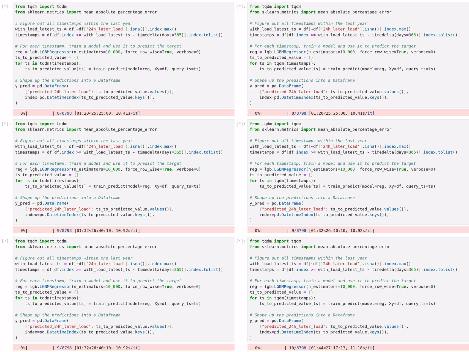
What can we do? Well, one way to address this issue is to subsample the testing timestamps, and use that as a test set. That way, our MAPE over the year will be an estimate of the actual MAPE.

from random import sample
import numpy as np

# Subsample to only train <N_TIMESTAMPS_TO_CONSIDER> models
timestamps = sample(timestamps, k=<N_TIMESTAMPS_TO_CONSIDER>)

To motivate this approach, let’s check that this estimate isn’t too far off the actual MAPE value by training a smaller model – a LightGBM with only 1 estimator – on all timestamps – making it 8760 models – and then computing the yearly-MAPE with varying amounts of discarded timestamps.

Study the impact of estimating the MAPE through timestamp subsampling

from tqdm import tqdm
from sklearn.metrics import mean_absolute_percentage_error
from random import sample

# Figure out all timestamps within the last year
with_load_latest_ts = df[~df['24h_later_load'].isna()].index.max() 
mask = (df.index <= with_load_latest_ts) & (df.index >= with_load_latest_ts - timedelta(days=365)) 
timestamps = df[mask].dropna(subset=('24h_later_load')).index.tolist()

# Subsample to only train 100 models
# timestamps = sample(timestamps, k=100)

# For each timestamp, train a model and use it to predict the target
reg = lgb.LGBMRegressor(n_estimators=1, force_row_wise=True, verbose=0)
ts_to_predicted_value = {}
for ts in tqdm(timestamps):
    ts_to_predicted_value[ts] = train_predict(model=reg, Xy=df, query_ts=ts)

# Shape up the predictions into a Dataframe
y_pred = pd.DataFrame(
    {"predicted_24h_later_load": ts_to_predicted_value.values()},
    index=pd.DatetimeIndex(ts_to_predicted_value.keys()),
)

# Get randomly-ordered timestamps to study the MAPE
random_timestamps = y_pred.index.tolist()
np.random.shuffle(random_timestamps) 

# Package the y_pred and y_true into a dataframe
y_true = df.loc[y_pred.index, ['24h_later_load']]
y_df = pd.concat([y_true, y_pred], axis=1)
y_df['APE'] = y_df.apply(lambda row: 100 * abs(row['24h_later_load'] - row['predicted_24h_later_load']) / row['24h_later_load'], axis=1)

# For each discarded proportion, compute the MAPE
discarded_proportion_to_mape = {}
for i in tqdm(range(len(random_timestamps))):
    discarded_proportion = i / len(random_timestamps) * 100
    discarded_proportion_to_mape[discarded_proportion] = y_df.loc[random_timestamps[i:], 'APE'].mean()

mape_df = pd.DataFrame({
    'discarded_proportion': discarded_proportion_to_mape.keys(),
    'estimated_MAPE': discarded_proportion_to_mape.values(),
})

# Plot
fig = px.line(
    mape_df, x='discarded_proportion', y='estimated_MAPE', 
    title='Evolution of the yearly-MAPE <br>when discarding some proportion of the timestamps making up the year',
    labels={'discarded_proportion': 'Proportion of discarded timestamps [%]', 'estimated_MAPE': 'Estimated MAPE [%] over the last year'}
)

fig.add_hline(y=mape_df.loc[0].estimated_MAPE, line_dash="dot",
              annotation_text="Actual MAPE", 
              annotation_position="bottom right")

Wonderful! As we hoped, we can get away with only sampling 10% of the data and still having our estimated MAPE be close (within 10%) of the actual MAPE.

Let’s go back to training our LightGBM model, this time judging it on 1% of the data, i.e. 87 samples:

Yearly-MAPE [%]	Model
10.8	ENTSO-E forecast
8.97	Dummy baseline
8.47 (estimated w/ 1% of timestamps)	LightGBM w/ 24h-ago-load

Great, on par with our dummy baseline. Let’s do better.

Leveraging more timestamps

Currently, the only load-related information our model can use is the 24h-ago-load; how about enrich our data with more timesteps?

# Enrich the data w/ more past loads
df['1h_ago_load'] = df['24h_later_load'].shift(24 + 1)
df['2h_ago_load'] = df['24h_later_load'].shift(24 + 2)
df['3h_ago_load'] = df['24h_later_load'].shift(24 + 3)
df['7d_ago_load'] = df['24h_later_load'].shift(24 + 24*7)
df.head(3)

Yearly-MAPE [%]	Model
10.8	ENTSO-E forecast
8.97	Dummy baseline
8.47 (estimated w/ 1% of timestamps)	LightGBM w/ 24h-ago-load
7.98 (estimated w/ 1% of timestamps)	LightGBM w/ several past loads

Even better! Let’s dive deeper and further improve our model.

Leveraging time attributes

Currently, our model treats all rows as identical, regardless of whether it’s midnight or noon, sunday or wednesday, june or december. There might be relevant predictive power in this information, so let’s enrich our data with this sense of “when” we are.

# Enrich the df with the datetime attributes
df['month'] = df.index.month
df['day'] = df.index.day
df['hour'] = df.index.hour
df['weekday'] = df.index.weekday
df.head(3)

Yearly-MAPE [%]	Model
10.8	ENTSO-E forecast
8.97	Dummy baseline
8.47 (estimated w/ 1% of timestamps)	LightGBM w/ 24h-ago-load
7.98 (estimated w/ 1% of timestamps)	LightGBM w/ several past loads
5.40 (estimated w/ 1% of timestamps)	LightGBM w/ several past loads & datetime attributes

That’s great! Can we fly higher?

Leveraging past load statistics

Using specific timesteps as features works great – apparently – but what if this specific timestep had a “weird” load? The model would then be skewed and underperform. One way to address this is to consider load statistics over different timespans.

# Compute statistics over the past 8h
df['8h_min'] = df['1h_ago_load'].rolling(window=8, min_periods=1).apply(np.nanmin)
df['8h_max'] = df['1h_ago_load'].rolling(window=8, min_periods=1).apply(np.nanmax)
df['8h_median'] = df['1h_ago_load'].rolling(window=8, min_periods=1).apply(np.nanmedian)

# Compute statistics over the past 24h
df['24h_min'] = df['1h_ago_load'].rolling(window=24, min_periods=1).apply(np.nanmin)
df['24h_max'] = df['1h_ago_load'].rolling(window=24, min_periods=1).apply(np.nanmax)
df['24h_median'] = df['1h_ago_load'].rolling(window=24, min_periods=1).apply(np.nanmedian)

# Compute statistics over the past 7d
df['7d_min'] = df['1h_ago_load'].rolling(window=24*7, min_periods=1).apply(np.nanmin)
df['7d_max'] = df['1h_ago_load'].rolling(window=24*7, min_periods=1).apply(np.nanmax)
df['7d_median'] = df['1h_ago_load'].rolling(window=24*7, min_periods=1).apply(np.nanmedian)

Yearly-MAPE [%]	Model
10.8	ENTSO-E forecast
8.97	Dummy baseline
8.47 (estimated w/ 1% of timestamps)	LightGBM w/ 24h-ago-load
7.98 (estimated w/ 1% of timestamps)	LightGBM w/ several past loads
5.40 (estimated w/ 1% of timestamps)	LightGBM w/ several past loads & datetime attributes
4.11 (estimated w/ 1% of timestamps)	LightGBM w/ several past loads & datetime attributes & past load statistics

Beautiful!

Conclusion

We now have a model performing at a satisfactory standard – estimated MAPE of 4.11% over the last year. We could of course continue improving – picking our features and hyper-parameters in a more robust and scientific manner¹¹, but for now, let’s move onto our next challenge: making our solution available to the user.

As I would figure out later, forecasts are usually added to the ENTSO-E website in bulk, at around 05:41 in the morning. Still, we picked this approach and are sticking with it. It is interesting to note that I assumed that’s how they generated their predictions, and should have asked them directly via email – as outlined in the motivation part of this writeup. ↩↩
We all know that itch. ↩
When I talk about complexity here, I don’t mean amount of parameters – although it is usually correlated – but complexity of the overall ML lifecycle of our approach. We are building a full-fledged solution – along with tooling to maintain, fix and update our solution. Its complexity goes beyond how many fake-neurons our model has. ↩
If that’s what you want to do, academy/research has a higher density of such problem statements. ↩
Here we talk about performance as if it was uni-dimensional. It rarely is. You should consider – amongst other things – the raw performance, the inference time, the ease of maintenance, the explainability, the upfront training cost and the deployment cost. ↩
I am by far not the first person to make that point – with KISS being one example of it – but it’s so easy to forget that I think it’s important to hammer it in. ↩
For tabular data, gradient-boosted-trees-based approaches often performs on par with – if not above – much more complex approaches (NN-based approaches of all flavors). ↩↩
The assumption that the train data is representative of the test data is also usually made – silently – but any mismatch would “only” translate into a low-performing model (on the test set), i.e. we would be aware of how the model would perform in the wild. ↩
By time-sensitive, I mean any kind of data gathered through time. It does not really matter if the actual time is part of the features, because seemingly-non-time-related features might contain time-related informations. If that is the case, the model might infer the time-data from these features – even just partially – and break once in production where it won’t be able to leverage it in the same way. ↩
24 * 365 == 8760 ↩
To select hyper-parameters – and features – optuna is a great optimization framework. To better understand how the selected features matter to the model, SHAP is a wonderful model-agnostic framework. ↩